Medical Data Analytics Using R

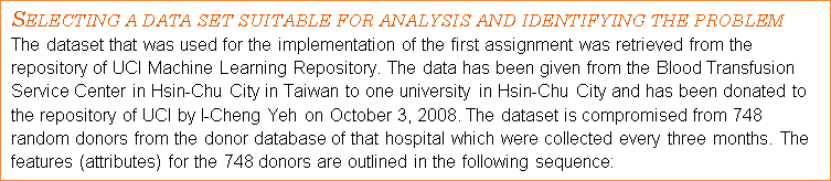
1.) R for Recency => months since last donation, 2.) F for Frequency => total number of donation, 3.) M for Monetary => total amount of blood donated in c.c., 4.) T for Time => months since first donation and 5.) Binary variable => 1 -> donated blood, 0-> didn’t donate blood.

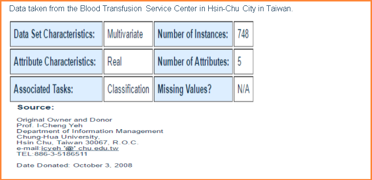
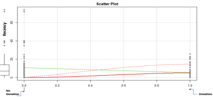
The main idea behind this dataset is the concept of relationship management CRM. Based on three metrics: Recency, Frequency and Monetary (RFM) which are 3 out of the 5 attributes of the dataset, we would be able to predict whether a customer is likely to donate blood again based to a marketing campaign. For example, customers who have donated or visited more currently (Recency), more frequently (Frequency) or made higher monetary values (Monetary) are more likely to respond to a marketing effort. Customers with less RFM score are less likely to react. It is also known in customer behavior, that the time of the first positive interaction (donation, purchase) is not significant. However, the Recency of the last donation is very important.

In the traditional RFM implementation each customer is ranked based on his RFM value parameters against all the other customers and that develops a score for every customer. Customers with bigger scores are more likely to react in a positive way for example (visit again or donate). The model constructs the formula which could predict the following problem.

• Keep in repository only customers that are more likely to continue donating in the future and remove those who are less likely to donate, given a certain period of time. The previous statement also determines the problem which will be trained and tested in this project.

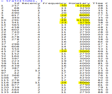
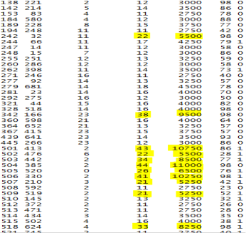
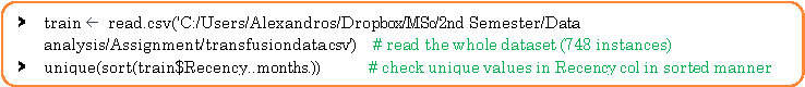
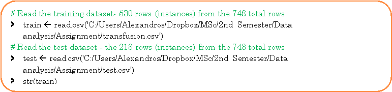Firstly, I created a .csv file and generated 748 unique random numbers in Excel in the domain [1,748] in the first column, which corresponds to the customers or users ID. Then I transferred the whole data from the .txt file (transfusion.data) to the .csv file in excel by using the delimited (‘,’) option. Then I randomly split it in a train file and a test file. The train file contains the 530 instances and the test file has the 218 instances. Afterwards, I read both the training dataset and the test dataset.

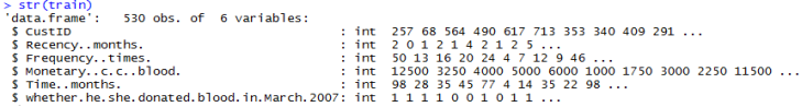
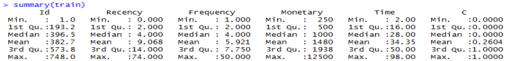
From the previous results, we can see that we have no missing or invalid values. Data ranges and units seem reasonable.

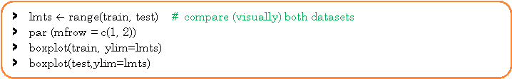
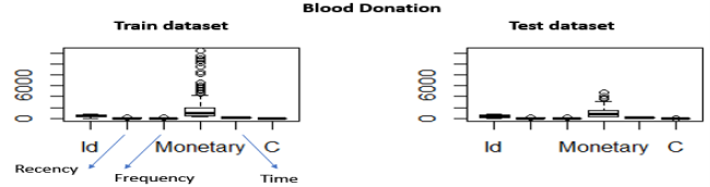
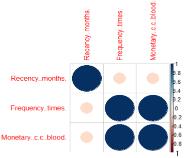
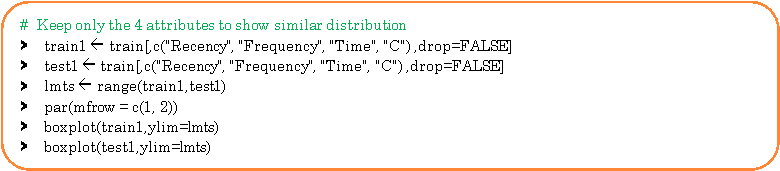
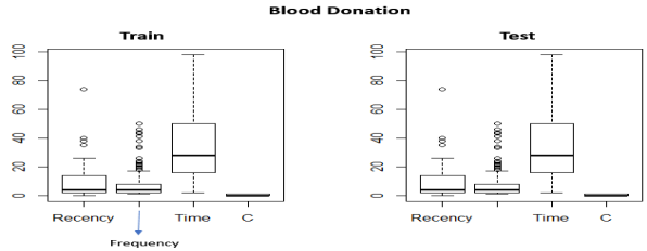
Figure 1 above depicts boxplots of all the attributes and for both train and test datasets. By examining the figure, we notice that both datasets have similar distributions and there are some outliers (Monetary > 2,500) that are visible. The volume of blood variable has a high correlation with frequency. Because the volume of blood that is donated each time is fixed, the Monetary value is proportional to the Frequency (number of donations) each person gave. For example, if the amount of blood drawn in each person was 250 ml/bag (Taiwan Blood Services Foundation 2007) March then Monetary = 250*Frequency. This is also why in the predictive model we will not consider the Monetary attribute in the implementation. So, it is reasonable to expect that customers with higher frequency will have a lot higher Monetary value. This can be verified also visually by examining the Monetary outliers for the train set. We retrieve back 83 instances.

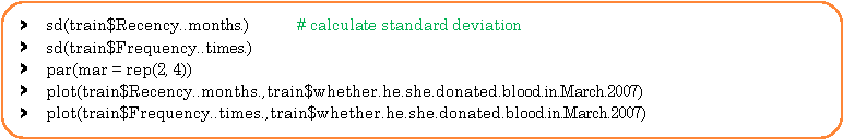
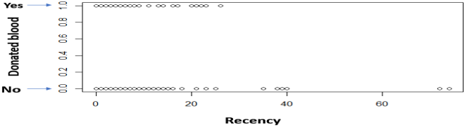
In order, to understand better the statistical dispersion of the whole dataset (748 instances) we will look at the standard deviation (SD) between the Recency and the variable ‘whether customer has donated blood’ (Binary variable) and the SD between the Frequency and the Binary variable.The distribution of scores around the mean is small, which means the data is concentrated. This can also be noticed from the plots.

From this correlation matrix, we can verify what was stated above, that the frequency and the monetary values are proportional inputs, which can be noticed from their high correlation.

Another observation is that the various Recency numbers are not factors of 3. This goes to opposition with what the description said about the data being collected every 3 months. Additionally, there is always a maximum number of times you can donate blood per certain period (e.g. 1 time per month), but the data shows that.

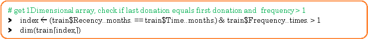
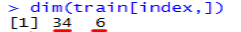
36 customers donated blood more than once and 6 customers had donated 3 or more times in the same month.

The features that will be used to calculate the prediction of whether a customer is likely to donate again are 2, the Recency and the Frequency (RF). The Monetary feature will be dropped. The number of categories for R and F attributes will be 3. The highest RF score will be 33 equivalent to 6 when added together and the lowest will be 11 equivalent to 2 when added together. The threshold for the added score to determine whether a customer is more likely to donate blood again or not, will be set to 4 which is the median value. The users will be assigned to categories by sorting on RF attributes as well as their scores. The file with the donators will be sorted on Recency first (in ascending order) because we want to see which customers have donated blood more recently. Then it will be sorted on frequency (in descending order this time because we want to see which customers have donated more times) in each Recency category. Apart from sorting, we will need to apply some business rules that have occurred after multiple tests:

• For Recency (Business rule 1):

1. If the Recency in months is less than 15 months, then these customers will be assigned to category 3.
2. If the Recency in months is equal or greater than 15 months and less than 26 months, then these customers will be assigned to category 2.
3. Otherwise, if the Recency in months is equal or greater than 26 months, then these customers will be assigned to category 1

• And for Frequency (Business rule 2):

1. If the Frequency is equal or greater than 25 times, then these customers will be assigned to category 3.
2. If the Frequency is less than 25 times or greater than 15 months, then these customers will be assigned to category 2.
3. If the Frequency is equal or less than 15 times, then these customers will be assigned to category 1

RESULTS

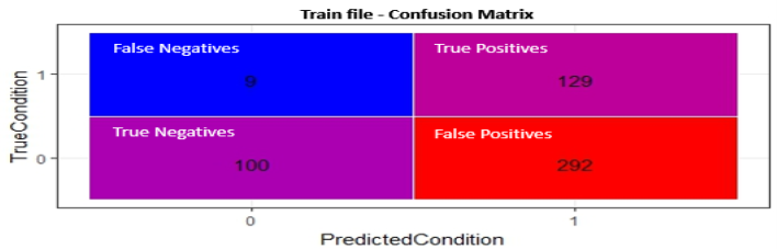
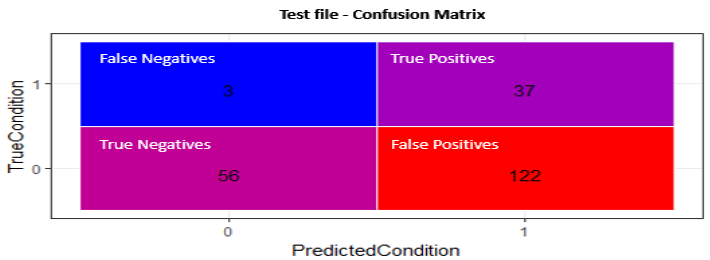
The output of the program are two smaller files that have resulted from the train file and the other one from the test file, that have excluded several customers that should not be considered future targets and kept those that are likely to respond. Some statistics about the precision, recall and the balanced F-score of the train and test file have been calculated and printed. Furthermore, we compute the absolute difference between the results retrieved from the train and test file to get the offset error between these statistics. By doing this and verifying that the error numbers are negligible, we validate the consistency of the model implemented. Moreover, we depict two confusion matrices one for the test and one for the training by calculating the true positives, false negatives, false positives and true negatives. In our case, true positives correspond to the customers (who donated on March 2007) and were classified as future possible donators. False negatives correspond to the customers (who donated on March 2007) but were not classified as future possible targets for marketing campaigns. False positives correlate to customers (who did not donate on March 2007) and were incorrectly classified as possible future targets. Lastly, true negatives which are customers (who did not donate on March 2007) and were correctly classified as not plausible future donators and therefore removed from the data file. By classification we mean the application of the threshold (4) to separate those customers who are more likely and less likely to donate again in a certain future period.

Lastly, we calculate 2 more single value metrics for both train and test files the Kappa Statistic (general statistic used for classification systems) and Matthews Correlation Coefficient or cost/reward measure. Both are normalized statistics for classification systems, its values never exceed 1, so the same statistic can be used even as the number of observations grows. The error for both measures are MCC error: 0.002577  and Kappa error:  0.002808, which is very small (negligible), similarly with all the previous measures.

REFERENCES

1. UCI Machine Learning Repository (2008) UCI machine learning repository: Blood transfusion service center data set. Available at: http://archive.ics.uci.edu/ml/datasets/Blood+Transfusion+Service+Center (Accessed: 30 January 2017).
2. Fundation, T.B.S. (2015) Operation department. Available at: http://www.blood.org.tw/Internet/english/docDetail.aspx?uid=7741&pid=7681&docid=37144 (Accessed: 31 January 2017).

The Appendix with the code starts below. However the whole code has been uploaded on my Git Hub profile and this is the link where it can be accessed.

https://github.com/it21208/RassignmentDataAnalysis/blob/master/RassignmentDataAnalysis.R

• library(ggplot2)
• library(car)

 # read training and testing datasets

• traindata   read.csv(‘C:/Users/Alexandros/Dropbox/MSc/2nd Semester/Data analysis/Assignment/transfusion.csv’)
• testdata   read.csv(‘C:/Users/Alexandros/Dropbox/MSc/2nd Semester/Data analysis/Assignment/test.csv’)

# assigning the datasets to dataframes

• dftrain  data.frame(traindata)
• dftest  data.frame(testdata)
• sapply(dftrain, typeof)

# give better names to columns

• names(dftrain)[1]  “ID”
• names(dftrain)[2]  “recency”
• names(dftrain)[3]”frequency”
• names(dftrain)[4]”cc”
• names(dftrain)[5]”time”
• names(dftrain)[6]”donated”

#——————————————————

• names(dftest)[1]”ID”
• names(dftest)[2]”recency”
• names(dftest)[3]”frequency”
• names(dftest)[4]”cc”
• names(dftest)[5]”time”
• names(dftest)[6]”donated”

# drop time column from both files

• dftrain$time  NULL
• dftest$time  NULL

#  sort (train) dataframe on Recency in ascending order

• sorted_dftrain  dftrain[ order( dftrain[,2] ), ]

#  add column in (train) dataframe -  hold score (rank) of Recency for each customer

• sorted_dftrain[ , “Rrank”]  0

#  convert train file from dataframe format to matrix

• matrix_train  as.matrix(sapply(sorted_dftrain, as.numeric))

#  sort (test) dataframe on Recency in ascending order

• sorted_dftest  dftest[ order( dftest[,2] ), ]

#  add column in (test) dataframe -hold score (rank) of Recency for each customer

• sorted_dftest[ , “Rrank”]  0

#  convert train file from dataframe format to matrix

• matrix_test  as.matrix(sapply(sorted_dftest, as.numeric))

# categorize matrix_train and add scores for Recency – apply business rule

• for(i in 1:nrow(matrix_train)) {

if (matrix_train [i,2] < 15) {

     matrix_train [i,6]  3

} else if ((matrix_train [i,2] < 26) & (matrix_train [i,2] >= 15)) {

     matrix_train [i,6]  2

} else {  matrix_train [i,6]  1  }

      }

# categorize matrix_test and add scores for Recency – apply business rule

• for(i in 1:nrow(matrix_test)) {

if (matrix_test [i,2] < 15) {

     matrix_test [i,6]  3

} else if ((matrix_test [i,2] < 26) & (matrix_test [i,2] >= 15)) {

     matrix_test [i,6]  2

} else {  matrix_test [i,6]  1 }

      }

# convert matrix_train back to dataframe

• sorted_dftrain  data.frame(matrix_train)

# sort dataframe 1rst by Recency Rank (desc.) then by Frequency (desc.)

• sorted_dftrain_2 sorted_dftrain[order(-sorted_dftrain[,6], -sorted_dftrain[,3] ), ]

# add column in train dataframe- hold Frequency score (rank) for each customer

• sorted_dftrain_2[ , “Frank”]  0

# convert dataframe to matrix

• matrix_train  as.matrix(sapply(sorted_dftrain_2, as.numeric))

# convert matrix_test back to dataframe

• sorted_dftest  data.frame(matrix_test)

# sort dataframe 1rst by Recency Rank (desc.) then by Frequency (desc.)

• sorted_dftest2  sorted_dftest[ order( -sorted_dftest[,6], -sorted_dftest[,3] ), ]

# add column in test dataframe- hold Frequency score (rank) for each customer

• sorted_dftest2[ , “Frank”]  0

# convert dataframe to matrix

• matrix_test  as.matrix(sapply(sorted_dftest2, as.numeric))

#categorize matrix_train, add scores for Frequency

• for(i in 1:nrow(matrix_train)){

  if (matrix_train[i,3] >= 25) {

    matrix_train[i,7]  3

  } else if ((matrix_train[i,3] > 15) & (matrix_train[i,3] < 25)) {

    matrix_train[i,7]  2

  } else {  matrix_train[i,7]  1  }

         }

#categorize matrix_test, add scores for Frequency

• for(i in 1:nrow(matrix_test)){

  if (matrix_test[i,3] >= 25) {

    matrix_test[i,7]  3

  } else if ((matrix_test[i,3] > 15) & (matrix_test[i,3] < 25)) {

    matrix_test[i,7]  2

  } else {   matrix_test[i,7]  1  }

}

#  convert matrix test back to dataframe

• sorted_dftrain  data.frame(matrix_train)

# sort (train) dataframe 1rst on Recency rank (desc.) & 2^nd Frequency rank (desc.)

• sorted_dftrain_2  sorted_dftrain[ order( -sorted_dftrain[,6], -sorted_dftrain[,7] ), ]

# add another column for the Sum of Recency rank and Frequency rank

• sorted_dftrain_2[ , “SumRankRAndF”]  0

# convert dataframe to matrix

• matrix_train  as.matrix(sapply(sorted_dftrain_2, as.numeric))

#  convert matrix test back to dataframe

• sorted_dftest  data.frame(matrix_test)

# sort (train) dataframe 1rst on Recency rank (desc.) & 2^nd Frequency rank (desc.)

• sorted_dftest2  sorted_dftest[ order( -sorted_dftest[,6],  -sorted_dftest[,7] ), ]

# add another column for the Sum of Recency rank and Frequency rank

• sorted_dftest2[ , “SumRankRAndF”]  0

# convert dataframe to matrix

• matrix_test  as.matrix(sapply(sorted_dftest2, as.numeric))

# sum Recency rank and Frequency rank for train file

• for(i in 1:nrow(matrix_train))

{ matrix_train[i,8]  matrix_train[i,6] + matrix_train[i,7] }

# sum Recency rank and Frequency rank for test file

• for(i in 1:nrow(matrix_test))

{ matrix_test[i,8]  matrix_test[i,6] + matrix_test[i,7] }

# convert matrix_train back to dataframe

• sorted_dftrain  data.frame(matrix_train)

# sort train dataframe according to total rank in descending order

• sorted_dftrain_2  sorted_dftrain[ order( -sorted_dftrain[,8] ), ]

# convert sorted train dataframe

• matrix_train  as.matrix(sapply(sorted_dftrain_2, as.numeric))

# convert matrix_test back to dataframe

• sorted_dftest  data.frame(matrix_test)

# sort test dataframe according to total rank in descending order

• sorted_dftest2  sorted_dftest[ order( -sorted_dftest[,8] ), ]

# convert sorted test dataframe to matrix

• matrix_test  as.matrix(sapply(sorted_dftest2, as.numeric))

# apply business rule check & count customers whose score >= 4 and that Have Donated, train file

# check & count for all customers that have donated in the train dataset

• count_train_predicted_donations  0
• counter_train  0
• number_donation_instances_whole_train  0
• false_positives_train_counter  0

• for(i in 1:nrow(matrix_train)) {

  if ((matrix_train[i,8] >= 4) & (matrix_train[i,5] == 1)) {

    count_train_predicted_donations = count_train_predicted_donations + 1  }

if ((matrix_train[i,8] >= 4) & (matrix_train[i,5] == 0)) {

    false_positives_train_counter = false_positives_train_counter + 1}

  if (matrix_train[i,8] >= 4) {

      counter_train  counter_train + 1

    }

  if (matrix_train[i,5] == 1) {

    number_donation_instances_whole_train  number_donation_instances_whole_train + 1

  }

}

# apply business rule check & count customers whose score >= 4 and that Have Donated, test file

# check & count for all customers that have donated in the test dataset

• count_test_predicted_donations  0
• counter_test  0
• number_donation_instances_whole_test  0
• false_positives_test_counter  0
• for(i in 1:nrow(matrix_test)) {

  if ((matrix_test[i,8] >= 4) & (matrix_test[i,5] == 1)) {

    count_test_predicted_donations = count_test_predicted_donations + 1  }

if ((matrix_test[i,8] >= 4) & (matrix_test[i,5] == 0)) {

    false_positives_test_counter = false_positives_test_counter + 1}

  if (matrix_test[i,8] >= 4) {

      counter_test  counter_test + 1

    }

  if (matrix_test[i,5] == 1) {

     number_donation_instances_whole_test  number_donation_instances_whole_test + 1

   }

}

# convert matrix_train to dataframe

• dftrain  data.frame(matrix_train)

# remove the group of customers who are less likely to donate again in the future from train file

• dftrain_final  dftrain[c(1:counter_train),1:8]

# convert matrix_train to dataframe

• dftest  data.frame(matrix_test)

# remove the group of customers who are less likely to donate again in the future from test file

• dftest_final  dftest[c(1:counter_test),1:8]

# save final train dataframe as a CSV in the specified directory – reduced target future customers

• write.csv(dftrain_final, file = “C:UsersAlexandrosDropboxMSc2nd SemesterData analysisAssignmenttrain_output.csv”, row.names = FALSE)

#save final test dataframe as a CSV in the specified directory – reduced target future customers

• write.csv(dftest_final, file = “C:UsersAlexandrosDropboxMSc2nd SemesterData analysisAssignmenttest_output.csv”, row.names = FALSE)

#train precision=number of relevant instances retrieved / number of retrieved instances collect.530

precision_train   count_train_predicted_donations / counter_train

# train recall = number of relevant instances retrieved / number of relevant instances in collect.530

recall_train  count_train_predicted_donations / number_donation_instances_whole_train

# measure combines Precision&Recall is harmonic mean of Precision&Recall balanced F-score for # train file

f_balanced_score_train  2*(precision_train*recall_train)/(precision_train+recall_train)

# test precision

precision_test  count_test_predicted_donations / counter_test

# test recall

recall_test  count_test_predicted_donations / number_donation_instances_whole_test

# the balanced F-score for test file

f_balanced_score_test  2*(precision_test*recall_test)/(precision_test+recall_test)

# error in precision

error_precision  abs(precision_train-precision_test)

# error in recall

error_recall  abs(recall_train-recall_test)

# error in f-balanced scores

error_f_balanced_scores  abs(f_balanced_score_train-f_balanced_score_test)

# Print Statistics for verification and validation

• cat(“Precision with training dataset: “, precision_train)
• cat(“Recall with training dataset: “, recall_train)
• cat(“Precision with testing dataset: “, precision_test)
• cat(“Recall with testing dataset: “, recall_test)
• cat(“The F-balanced scores with training dataset: “, f_balanced_score_train)
• cat(“The F-balanced scores with testing dataset:  “, f_balanced_score_test)
• cat(“Error in precision: “, error_precision)
• cat(“Error in recall: “, error_recall)
• cat(“Error in F-balanced scores: “, error_f_balanced_scores)

# confusion matrix (true positives, false positives, false negatives, true negatives)

# calculate true positives for train which is the variable ‘count_train_predicted_donations’

# calculate false positives for train which is the variable ‘false_positives_train_counter’

# calculate false negatives for train

• false_negatives_for_train  number_donation_instances_whole_train – count_train_predicted_donations

# calculate true negatives for train

• true_negatives_for_train  (nrow(matrix_train) – number_donation_instances_whole_train) – false_positives_train_counter
• collect_trainc(false_positives_train_counter, true_negatives_for_train, count_train_predicted_donations, false_negatives_for_train)

# calculate true positives for test which is the variable ‘count_test_predicted_donations’

# calculate false positives for test which is the variable ‘false_positives_test_counter’

# calculate false negatives for test

• false_negatives_for_test  number_donation_instances_whole_test – count_test_predicted_donations

# calculate true negatives for test

• true_negatives_for_test(nrow(matrix_test)-number_donation_instances_whole_test)- false_positives_test_counter
• collect_test  c(false_positives_test_counter, true_negatives_for_test, count_test_predicted_donations, false_negatives_for_test)
• TrueCondition  factor(c(0, 0, 1, 1))
• PredictedCondition  factor(c(1, 0, 1, 0))

# print confusion matrix for train

• df_conf_mat_train  data.frame(TrueCondition,PredictedCondition,collect_train)
• ggplot(data = df_conf_mat_train, mapping = aes(x = PredictedCondition, y = TrueCondition)) +

  geom_tile(aes(fill = collect_train), colour = “white”) +

  geom_text(aes(label = sprintf(“%1.0f”, collect_train)), vjust = 1) +

  scale_fill_gradient(low = “blue”, high = “red”) +

  theme_bw() + theme(legend.position = “none”)

#  print confusion matrix for test

• df_conf_mat_test  data.frame(TrueCondition,PredictedCondition,collect_test)
• ggplot(data =  df_conf_mat_test, mapping = aes(x = PredictedCondition, y = TrueCondition)) +

  geom_tile(aes(fill = collect_test), colour = “white”) +

  geom_text(aes(label = sprintf(“%1.0f”, collect_test)), vjust = 1) +

  scale_fill_gradient(low = “blue”, high = “red”) +

  theme_bw() + theme(legend.position = “none”)

# MCC = (TP * TN – FP * FN)/sqrt((TP+FP) (TP+FN) (FP+TN) (TN+FN)) for train values

• mcc_train  ((count_train_predicted_donations * true_negatives_for_train) – (false_positives_train_counter * false_negatives_for_train))/sqrt((count_train_predicted_donations+false_positives_train_counter)*(count_train_predicted_donations+false_negatives_for_train)*(false_positives_train_counter+true_negatives_for_train)*(true_negatives_for_train+false_negatives_for_train))

# print MCC for train

• cat(“Matthews Correlation Coefficient for train: “,mcc_train)

# MCC = (TP * TN – FP * FN)/sqrt((TP+FP) (TP+FN) (FP+TN) (TN+FN)) for test values

• mcc_test  ((count_test_predicted_donations * true_negatives_for_test) – (false_positives_test_counter * false_negatives_for_test))/sqrt((count_test_predicted_donations+false_positives_test_counter)*(count_test_predicted_donations+false_negatives_for_test)*(false_positives_test_counter+true_negatives_for_test)*(true_negatives_for_test+false_negatives_for_test))

# print MCC for test

• cat(“Matthews Correlation Coefficient for test: “,mcc_test)

# print MCC err between train and err

• cat(“Matthews Correlation Coefficient error: “,abs(mcc_train-mcc_test))

# Total = TP + TN + FP + FN for train

• total_train  count_train_predicted_donations + true_negatives_for_train + false_positives_train_counter + false_negatives_for_train

# Total = TP + TN + FP + FN for test

•  total_test  count_test_predicted_donations + true_negatives_for_test + false_positives_test_counter + false_negatives_for_test

# totalAccuracy = (TP + TN) / Total – for train values

• totalAccuracyTrain  (count_train_predicted_donations + true_negatives_for_train)/ total_train

# totalAccuracy = (TP + TN) / Total – for test values

• totalAccuracyTest  (count_test_predicted_donations + true_negatives_for_test)/ total_test

# randomAccuracy = ((TN+FP)*(TN+FN)+(FN+TP)*(FP+TP)) / (Total*Total)  for train values

• randomAccuracyTrain((true_negatives_for_train+false_positives_train_counter)*(true_negatives_for_train+false_negatives_for_train)+(false_negatives_for_train+count_train_predicted_donations)*(false_positives_train_counter+count_train_predicted_donations))/(total_train*total_train)

# randomAccuracy = ((TN+FP)*(TN+FN)+(FN+TP)*(FP+TP)) / (Total*Total)  for test values

• randomAccuracyTest((true_negatives_for_test+false_positives_test_counter)*(true_negatives_for_test+false_negatives_for_test)+(false_negatives_for_test+count_test_predicted_donations)*(false_positives_test_counter+count_test_predicted_donations))/(total_test*total_test)

# kappa = (totalAccuracy – randomAccuracy) / (1 – randomAccuracy) for train

• kappa_train  (totalAccuracyTrain-randomAccuracyTrain)/(1-randomAccuracyTrain)

# kappa = (totalAccuracy – randomAccuracy) / (1 – randomAccuracy) for test

• kappa_test  (totalAccuracyTest-randomAccuracyTest)/(1-randomAccuracyTest)

# print kappa error

• cat(“Kappa error: “,abs(kappa_train-kappa_test))